
7 posts tagged with "llms-in-production"

View All Tags

· 17 min read
Hamish Hall

Massively parallel hardware accelerators, such as GPUs, have played a key role in providing the computational power required to train modern machine learning models, especially recent Large Language Models (LLMs). Training these models can still take several months, regardless of the amount of resources allocated to them. The problems, however, don't stop at training - these models are so large and unwieldy that just interacting with and inferring from them can also be a challenge. This is particularly pertinent for language modelling use cases which need almost real-time responses to not frustrate users - no one wants to talk to a chatbot that takes a few seconds to send each word. Now imagine how tricky this gets as you scale your application to thousands of concurrent users! Fortunately, in these situations where the models are too big or the request traffic too high, we can turn back to the same hardware that built these models in the first place: large, massively parallel clusters of GPUs.

Distributed computing

To truly appreciate the benefits of multi-gpu inference, we need to understand some of the fundamentals of distributed computing.

Amdahl’s law and the limits of parallelisation

To begin, we need to start with a reality check on the computational speed ups available to us through parallelisation. Equation 1 is Amdahl’s law, and relates the fraction of our program that can be parallelised with the number of parallel nodes we have available, to calculate our potential speed up. This speed up is a theoretical limit as it doesn’t include any communication costs between our processes, which will apply heavily in our multi-gpu environment for result reconciliation and aggregation.


Speedup(S)<=1(1f)+fN\mathrm{Speedup}(S) <= \frac{1}{{(1 - f) + \frac{f}{N}}}

Equation 1:

SS
is the theoretical speedup,
ff
is the fraction of our program that can be parallelised and
NN
is the number of nodes we have to parallelise across.

Amdahl's law
Fig 1: Visualisation of how the nature of our program dictates how we can parallelise it.

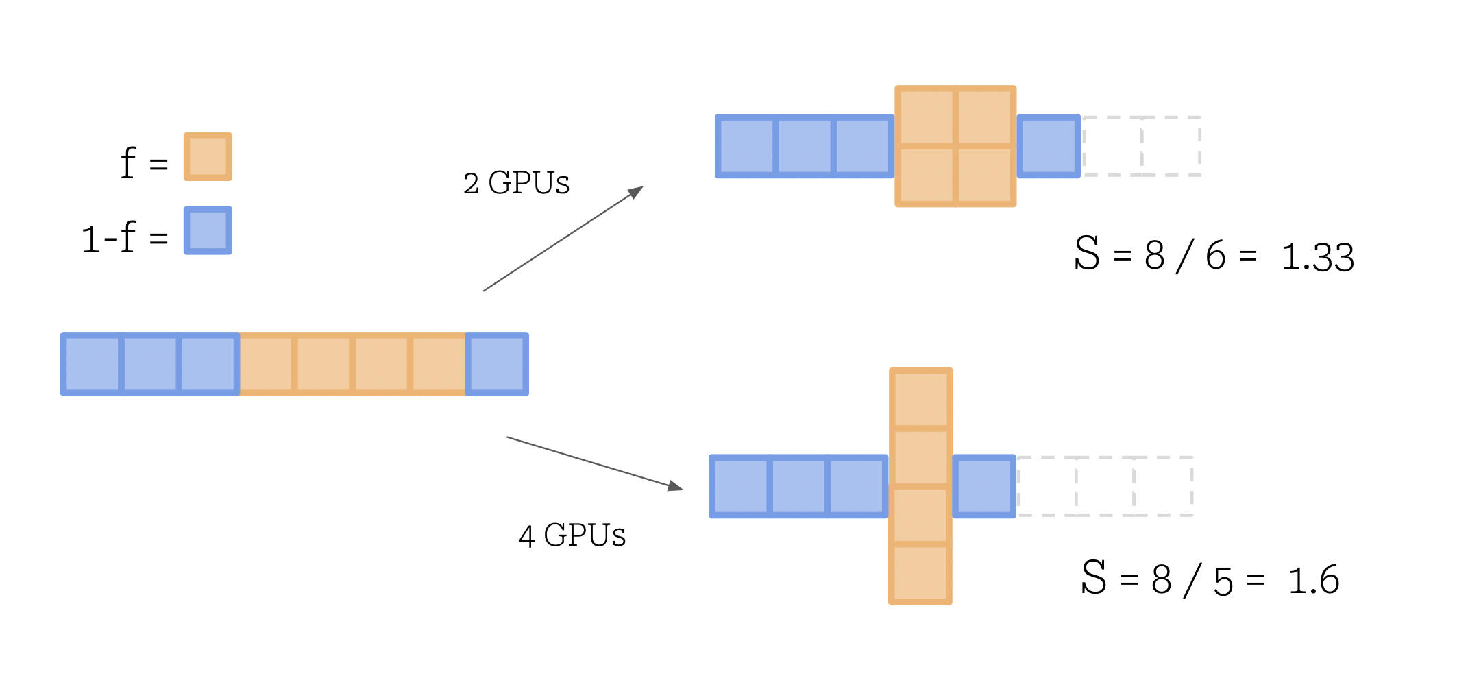
Here we visualize distributing our ML program across a number of parallel devices. Parts of the program (in blue) must inevitably run in series, such as data retrieval and preprocessing, initialising the parallel nodes and closing the program with some postprocessing. Likewise, the orange blocks represent computations that can happen simultaneously, such as passing a single input through our model, and we are capped by our available nodes as to how many units can run simultaneously. If these units exceed our number of devices, they must execute consecutively on our devices.

This means using the absolute theoretical limit, when splitting our program over 2 GPUs, we cannot expect to pass the limit of half of the original time taken - and should expect a time somewhat greater than this due to the serial parts of our program, pre- and post-processing, plus the communication overheads required between our parallel processes.

So, while any speed up is good news, to appreciate the real appeal of stacking our GPUs, we need to segue into some more inference metrics.

Latency vs. Throughput

Latency and throughput are two fundamental performance metrics used to grade computing systems, and while we usually want competitive values in both, our use case can prioritise one over the other.

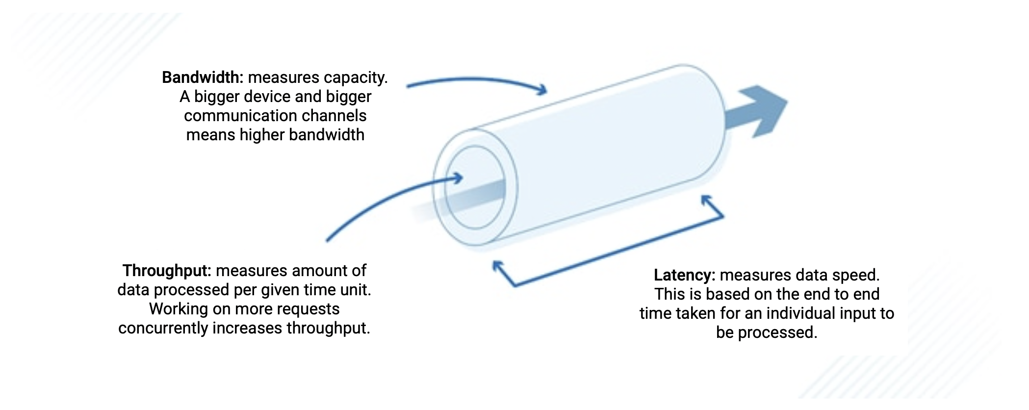
  • Latency: often referred to as response time, measures the time it takes for a single unit of data to traverse a system from source to destination - in the context of our LLMs this is the time we see between each subsequent token returning from our models.
  • Throughput: on the other hand, quantifies the rate at which data can be processed or transmitted within a given time frame - for our LLMs this value describes our output tokens per second. Higher throughput indicates our system's ability to handle a larger volume of requests efficiently.
latency vs thoughput
Fig 2: Latency vs. Throughput vs. Bandwidth.

While these two values may appear similar and are, in fact, inherently interconnected (reducing latency typically leads to increased throughput), there are subtle ways we can tweak them individually.

  • Batch size: LLMs consist of numerous consecutive matrix multiplications, and when processed on massively parallel devices like GPUs, the time required to handle a batch of inputs through these operations is negligibly increased compared to a single input (to an extent). See Fig 3: if we can process multiple inputs simultaneously, at low cost to the execution time, we can multiply the tokens passing through and outputting from our model per unit time - this is a big boost to our throughput. (Note: on a sequential processor like a CPU, these steps have to execute consecutively and you lose the benefit).
a diagram of matrix multiplication
Fig 3: GPUs parallelise matrix multiplication by tiling the input matrices and processing them simultaneously in individual threads. If matrix A is our batches of inputs, B our weights, and each tile runs concurrently, we can get a lot extra computation done in the same time by increasing our batch size (height of A) with just a small cost to recompose the output from the sub units.
  • Quantization: a lot of time is spent moving large chunks of data around to be processed in a system with limited bandwidth, causing queues and bottlenecks. One of the big advantages to quantizing our models, apart from allowing use of bigger models, is massively reducing the size of our data, and increasing the speed it can be transferred. This is a win for latency.
  • Caches: There are many repetitious calculations that occur during the inference process, and if we can store the results of these calculations in a cache, we can save time by not having to recompute them. This is a win for latency, and improves our throughput in the process.

To summarize, latency measures speed and throughput measures volume - and the latter is where we're going to see our dramatic results! Bigger batch sizes is a significant opportunity for boosting our throughput, and allowing our deployed model to serve many users concurrently while keeping performance competitive. The problem is these batches need space to work with:

Fitting a model (and some space to work with) on our device

Firstly, lets calculate the raw size of our model:

Size (in Gb) = Parameters (in billions) * Size of data (in bytes)\text{Size (in Gb) = Parameters (in billions) * Size of data (in bytes)}

And let’s see how these numbers look for some of the most popular models:

Modelfp32fp16int8
OPT-1.3b5.22.61.3
Llama2-7b28.014.07.0
Llama2-13b52.026.013.0
Flan-T5-L3.11.60.8
Flan-T5-XL12.06.03.0
BERT-L1.20.60.3
BERT-XL5.22.61.3

Table 1: Model sizes in Gb for different precisions.

Our first imperative for working with GPUs is that the model itself needs to be able to fit within the devices’ VRAM. So looking at the following range of common GPUs, we can see that for a Llama-7b at fp16, some GPUs are inaccessible and for Llama-13b at fp16 all but the A100s are unusable, unless we can find a way to split the model across more than one device. So our first lesson: for large models, it may be a necessity to split it across a multi-gpu backend just to be able to run it. GPU prices also grow exponentially with their size, so chances are you are more likely to be able to afford multiple smaller GPUs than a single large one.

GPUVRAM
306012
V10016
409024
A1024
A10040/80

Table 2: GPU memory capacity in Gb.

Next we need to think about how much extra space we need reserved for our rolling calculations. There is a back of the envelope esimate1 that for a 13b parameter model, each token requires 1mb of additional space for continuous values. So a prompt of 128 tokens, with a desired generation of 128 tokens will require 256mb of additional space. This seems like a low amount, but that means a batch size of 48 would max out our 3060 GPU without even the model present!

But to increase our throughput and the amount of users we can serve concurrently, we know we need to up our batch size. This is the next argument for splitting our model across GPUs: it leaves more space on each device for running the inference on an increased amount of inputs.

Strategies for distributing across multiple gpus

There are a couple of ways we can approach our multi-gpu environment:

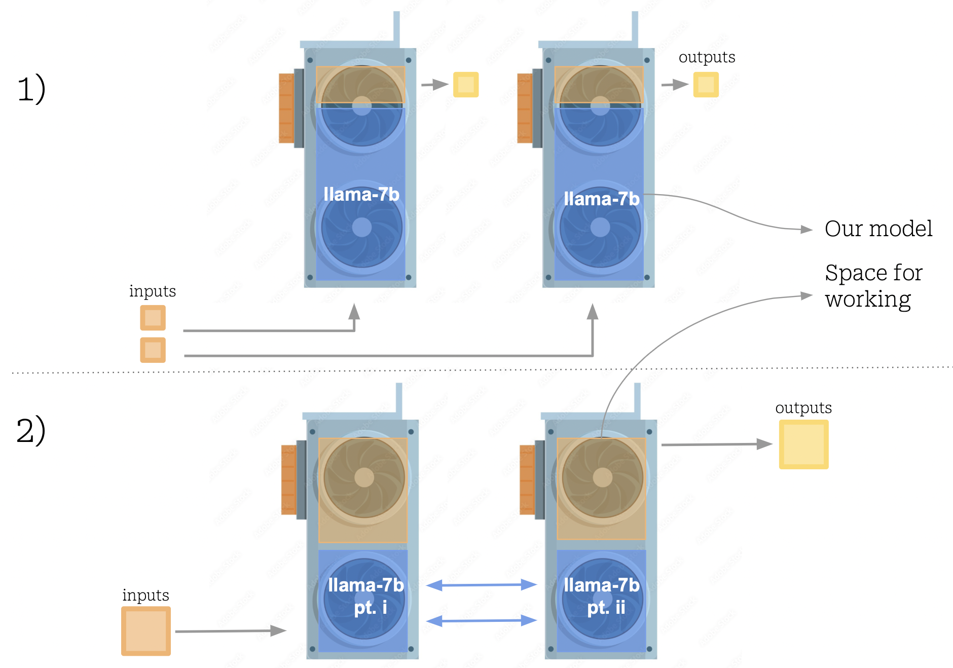
  1. Repeat our model on multiple devices: this is the simplest approach, and will afford us throughput increases without any inter-gpu communication costs. The technique involves simply loading the model individually onto each of our GPUs, and using a queue system to distribute incoming requests to each of the models. The main advantage to this approach is simplicity, but some downsides are evident. For one, there is a lot of redundant information wasting precious GPU space by repeating the same weights across all the devices. This approach also stuffs a large model into each GPU, reducing the capacity left to fit in our runtime data, forcing us to operate at lower batch sizes.

  2. Split our model: the alternative is to chunk our model and split it across the devices. This way is much more complex to code, and also comes with some communication overheads, as the model needs to costantly combine calculation outputs before moving on to the next stage. However, this way allows us to access massive models that can't normally fit on our available hardware, and also allows us to operate at much larger batch sizes, as we have more space to work with on each device.

The latter approach is particularly exciting: it is known that large models typically outperform their smaller counterparts, so if we can use our distributed hardware to unlock previously inaccessible models like llama-13b then this is a big win.

Comparing multiple replicas to a sharded model.
Fig 4: Multiple replicas of a model vs. a sharded model.

How to split a model: pipeline vs tensor (vs data) parallelism

Data parallelism is option 1) in the previous section, whereby different chunks of our data are processed in parallel on replicas of the model. For reasons previously discussed, we wish to split our model across our devices and there are a few ways we can achieve this, the most common being pipeline or tensor parallelism.

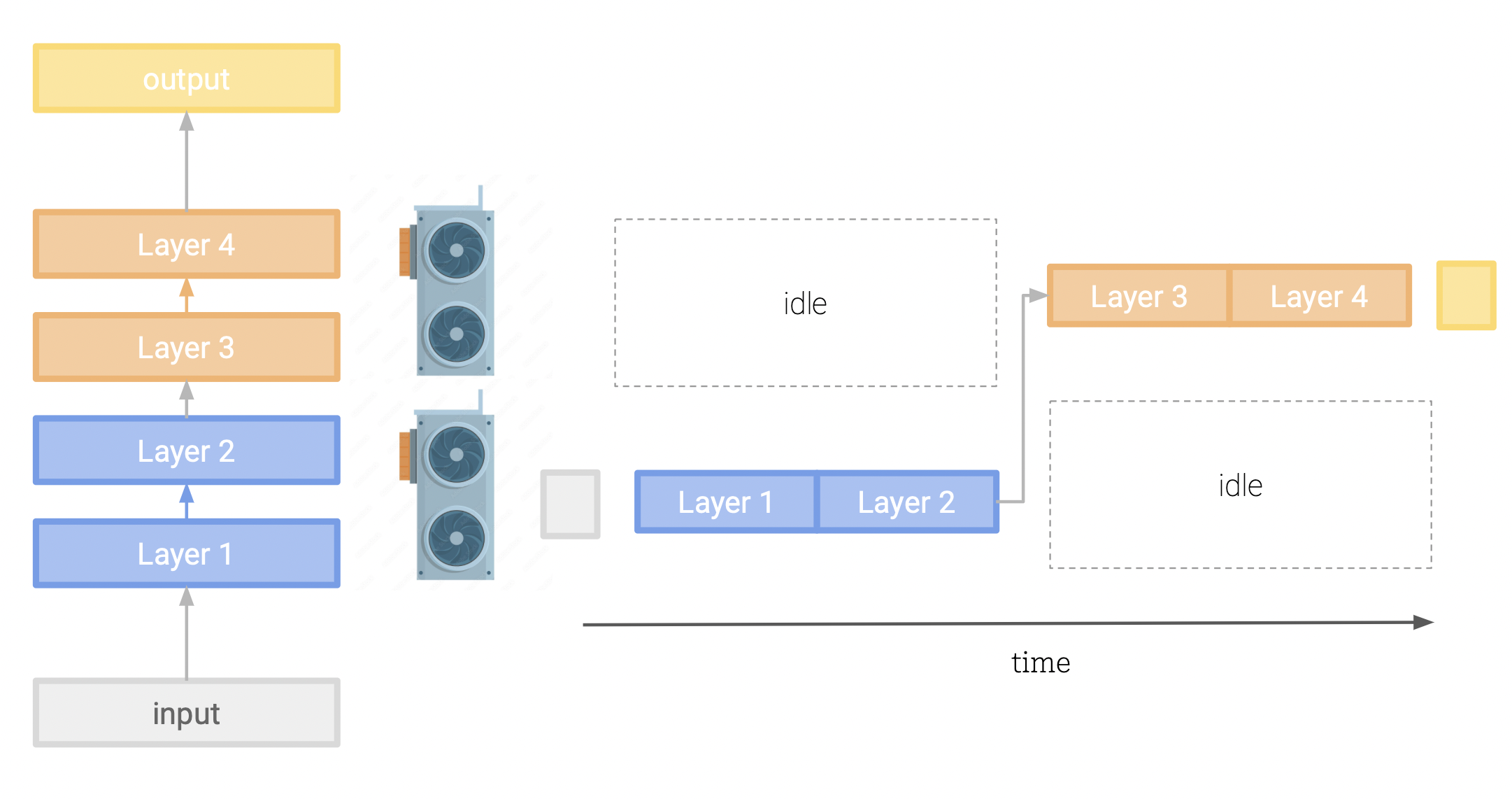
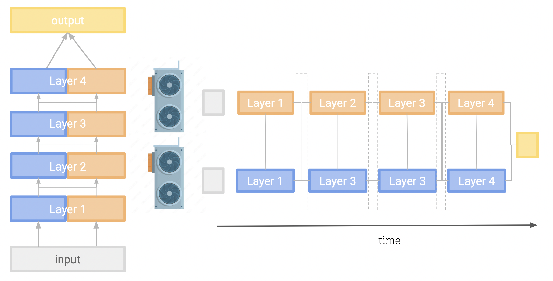
Pipeline parallelism:

This involves splitting our model layers across our devices. After one device has finished processing its chunk of the model, it passes the intermediate values to the next device to continue the computation. While this is a simple approach, it is limited by the sequential nature of the model, and the fact that the each device must wait for the previous to finish before it can move on to the next layer. This means both devices can sit idle for a large portion of the time, while the other is processing. We have managed to split our model across devices, but have lost our parallel execution.
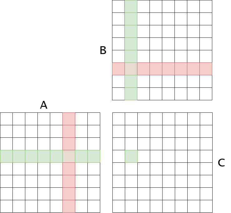
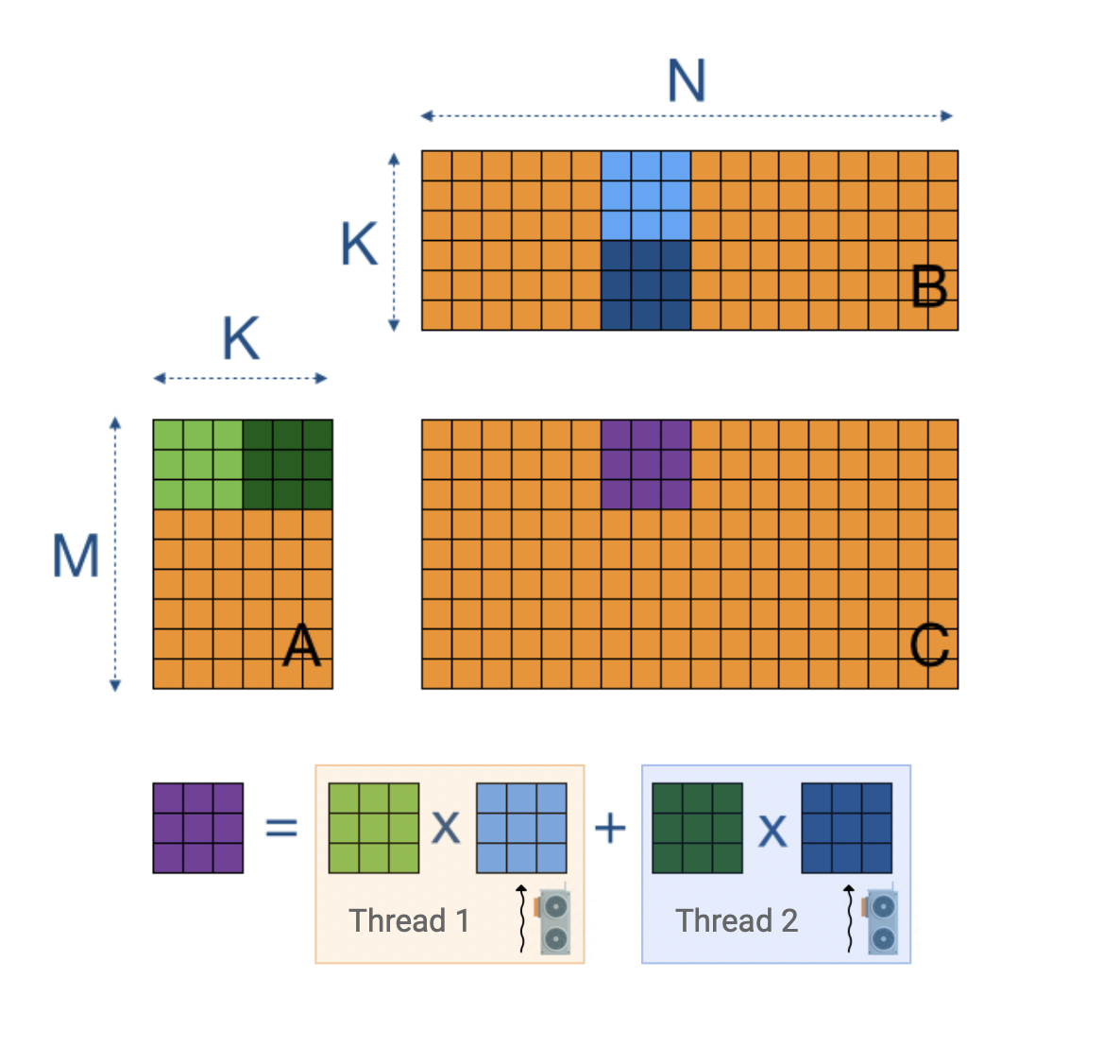
a diagram of pipeline parallelism
Fig 5: Pipeline parallelism.

Tensor parallelism:

Someone smart noticed the above approach was underutilizing the GPUs because of bubbles of idle wait time in their computation graphs. To maximise the computation occuring, ideally we want our GPUs operating as close to 100% utilization as possible for as much time as possible. We can achieve this by splitting our model in a slightly more ingenious way. Instead of splitting our model by layer, we split up the large matrices internal to our layers such as the big MLPs or attention modules. Different parts of the output matrix can be calcuated simultaneously and the intermediate tensors concated for the full result. As you can see in the following diagram this calculation is equivalent so no results are compromised.

Matrix multiplication can be done in parts and then recombined
Fig 6: Matrix multiplications can be done in parts and recombined for the same result.

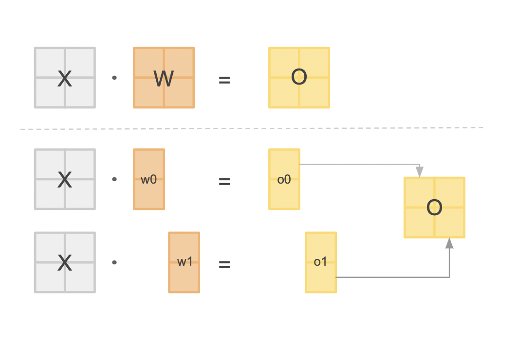
By following this method we can have all of our devices crunching away on heavy computation (what they are best at) at all times, at the cost of some communication overheads to synchronize tensors. Despite its added complexity, tensor parallelism is the way to go if you want ultra competitive performance from your multi-gpu setup.

Tensor parallism diagram
Fig 7. Tensor parallelism.

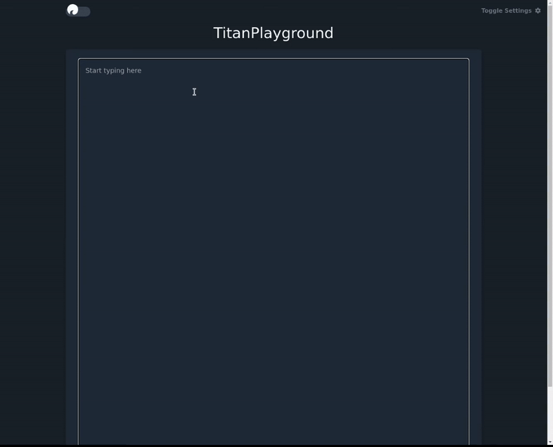
TitanML's multi-gpu engine

The above taster is a brief introduction to the complexities of distributed computing, and the challenges of deploying large models in production. Luckily, we at TitanML are on a mission to make this easier for you.
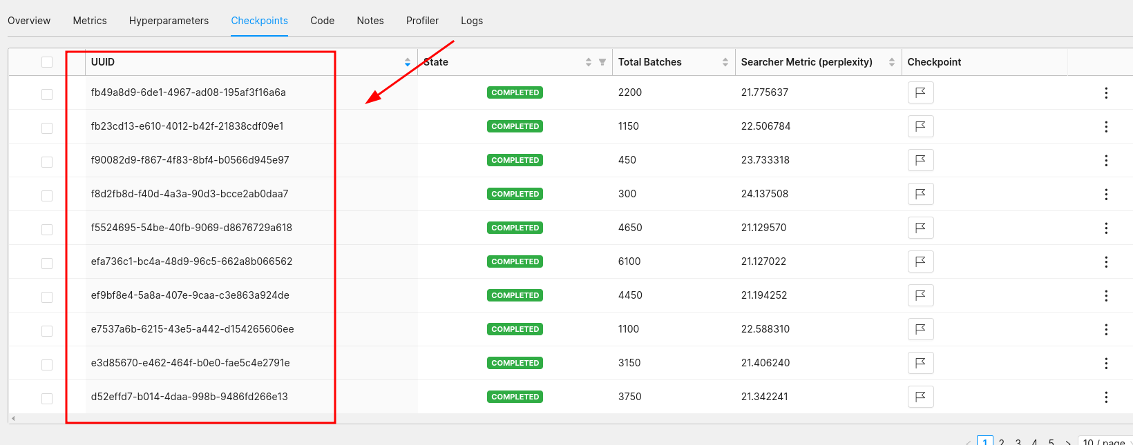
Results

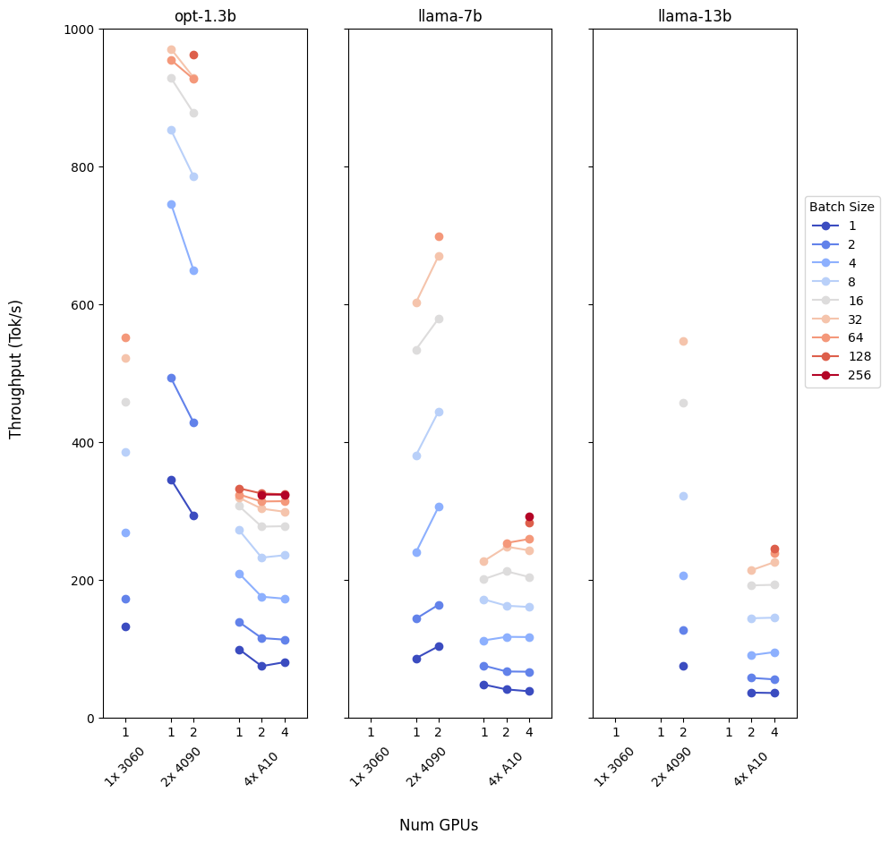
The following graph is a demonstration of the trials and tribulations of working with multiple GPUs. Its not as easy as just throwing more hardware at the problem, we need to assess and benchmark if its right for the type of application we are planning to build.

Inference throughput results table
Fig 8. Inference throughput achieved for different models on different GPU clusters, at different batch sizes.
paramvalue
prompt_length3
max_new_tokens256
min_new_tokens256
sampling_temperature1
sampling_topp0.9
sampling_topk20

Table 3: Generation parameters for repeatability.

Discussion

Off the bat, we can see that a multi-gpu environment is wasted for a small model. The communication overheads and the fact that the model can fit on a single device means we are better off just using a single GPU. The larger GPU can work with bigger batch sizes, but the token/s is so high for the single GPU, that the throughput is likely maintained just because of the very low latency. In this scenario, we are better off using the data parallel regime and using each GPU to host its own model.

Fig 8 also demonstrates to us how our model size can outright reject potential hardware setups - where datapoints are missing, the setup failed with dreaded Out of Memory(OOM) errors. As we can see, if you want to run a Llama-13b you're going to need more than 1 GPU.

The most dramatic effect of a 4 GPU cluster is unlocking the 256 batch size. The reduced throughput is a second hand effect of the slower latency within the cluster, but this does mean 256 individual users are receiving output simultaneously (even if at a slower rate than on the 4090s). This may be a tradeoff that is worth it for your application. Unless you are using some very exotic batching methods such as continuous or piggyback batching (coming to Titan soon!), your next set of requests will sit queuing while the current batch is being processed. Sometimes serving more requests concurrently, even if it seems like it lowers your throughput, can be necessary, as the total average wait time for the user is still lower - this depends on the wider context of your whole application architecture.

Do it yourself

Running a model distributed across multiple GPUs, with all the previously discussed optimizations, can be achieved using Titan Takeoff Server2 with a single command:

docker run
-e TAKEOFF_BACKEND=multi-gpu # Specify multi-gpu backend
-e TAKEOFF_MODEL_NAME=meta-llama/llama-2-13b # Specify which model
-e TAKEOFF_ACCESS_TOKEN=<token> # Needed for Llama-2 models
-e CUDA_VISIBLE_DEVICES=<'0,1...'> # Decide which of our GPUs to use
--num-gpus all # Let the docker container access these
--shm-size=2gb
-p 3000:3000 # Port forward
takeoff-pro:gpu # The takeoff pro image

You can now send inference requests to your model using the following command, and the takeoff runtime will handle distributing the inputs, the parallel computation and aggregating the results:

curl http://localhost:8000/generate_stream \
-X POST \
-N \
-H "Content-Type: application/json" \
-d '{"text": "List 3 things you can do in London"}'

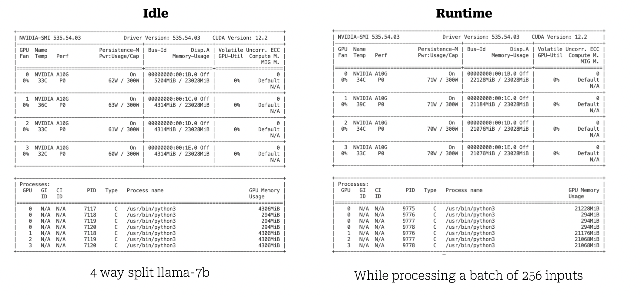
The text field can be an array of inputs with dimension matching your desired batch size, and the response will be an array of outputs of the same length. If you wish to watch your GPU utilisation during the process, you can run the following command in a separate terminal:

watch -n0.2 nvidia-smi

Here we can see what it looks like when our model is distributed across 4 devices, and how much memory a large batch size uses up!

A view of the outputs of the nvidia-smi command
Fig 9: GPU utilization during parallelized inference on a cluster of 4x A10s.

Further improvements
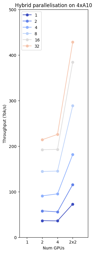
Hybrid approaches

The eagle eyed amongst you may have noticed that the gains going from 2 to 4 GPUs for the llama-13b model are not dramatic enough to really justify doubling our expensive hardware resources. But! We can use our 4 GPU cluster more wisely, combining both tensor parallelism and the previously discussed data parallelism to eke much better performance out of our setup. If we split our model across 2 GPUs, and replicate this setup twice we can utilise all 4 of our GPUs, and achieve almost double the throughput of a 4 way tensor parallel model.

Data and tensor parallelism
Fig 10: The best performance comes from a hybrid of tensor and data parallelism. Here we get the best throughput from our cluster by halving and distributing the Llama-13b on two devices and replicating this setup on the remaining 2 GPUs. Incoming requests are greedily taken off the queue by whichever cluster of the 2 is ready to process them.

For this, now even more complex situation, we at TitanML have got you covered again! With Takeoff we can manage control groups of clustered GPUs so your requests can all hit a single endpoint (our highly optimised rust server) and we will organise distributing these requests across multiple sets of GPUs, each holding split up models. Finding the optimal setup for your application can be a mixture of intuition and trial and error, but with Takeoff we do as much of the initialisation and orchestration as possible, so that you can focus on rapidly prototyping and benchmarking your options.

Happy hacking!

About TitanML

TitanML enables machine learning teams to effortlessly and efficiently deploy large language models (LLMs). Their flagship product Takeoff Inference Server is already supercharging the deployments of a number of ML teams.

Founded by Dr. James Dborin, Dr. Fergus Finn and Meryem Arik, and backed by key industry partners including AWS and Intel, TitanML is a team of dedicated deep learning engineers on a mission to supercharge the adoption of enterprise AI.

Footnotes

  1. https://github.com/ray-project/llm-numbers#v100-16gb-a10g-24gb-a100-4080gb-gpu-memory-capacities

  2. Multi-gpu support is currently a Pro feature - if you are interested, contact us here: https://www.titanml.co/contact

· 9 min read
Jamie Dborin

One of the most notable features of large language models (LLMs) is actually in the name - they are large (shocking, I know). Up to the very recent past, even models as large as 10B parameters were considered cumbersomely large, and inconvenient to work with.

Now, all of a sudden, these models are popping up on Raspberry Pi's, laptops, and even mobile phones. How did this happen? How did we go from multi-billion parameter models being solely in the realm of compute-rich tech companies to being run on the edge. The release of powerful open-source LLMs also kicked off a plethora of research into ways to optimize these models for inference. One particular avenue of research that has proven extremely fruitful involves the concept of quantization. In this blog post we are going to explain:

What is Quantization

Language models, especially the large ones, are often trained using either 32-bit or 16-bit precision. What this means is that each parameter in the model is represented with either 32 or 16 bits. When we talk about a 32-bit model, it's stored using 32-bit floating point numbers. On the other hand, 16-bit models employ 16-bit floating point numbers or the 16-bit bfloat (brain-float, named after Google Brain, where the data type was first conceived) data type.

Now, why does this bit precision matter? Well, in terms of storage, a 32-bit model requires 4GB of memory for every 1 Billion parameters. Meanwhile, a 16-bit model halves that requirement to 2GB for the same number of parameters. Remember, this calculation only accounts for the storage of the model. Running the model in real-time requires additional memory. Moreover, while executing a large language model, temporary values called 'activations' can be quantized. This isn't predominantly to save memory but to harness the speed of 8-bit matrix multiplication operations that modern CPUs and GPUs support. Although this post sheds some light on activation quantization, our main focus will be on weight-only quantization.

Quantization is essentially a method to reduce the bit storage required for each model parameter. A prevalent approach is to bring it down to 8 bits per parameter. By this logic, a model with 1 Billion parameters would need just 1GB of memory. Translating this, a model with 7 Billion parameters (like a 'Llama' model) would necessitate at least 7GB of memory. Such a memory footprint is manageable on high-end laptops, but could challenge the capabilities of contemporary smartphones.

To put this into perspective, the most memory-endowed iPhones offer around 6GB, while the Google Pixel phones max out at approximately 8GB. So, if our goal is to facilitate large language models (LLMs) on mobile devices, we must push quantization boundaries. How? By venturing into even tinier bit-widths—7, 6, 5, 4, 3, 2, or even just a single bit per parameter. For instance, at 4-bit precision, our 7B parameter 'Llama' model would consume only 3.5GB, making it viable for today's smartphones. But delving into these lower bit-widths introduces complications. Striking the right balance among model quality, speed, and size becomes a nuanced challenge.

The quantization formula to quantize to int8 looks like this:

WQ=WF×255MaxW_Q = \lfloor{\frac{W_F \times 255}{Max}}\rfloor

The Max parameter is a floating point number extracted from the weight to be quantized. 255 comes from the fact that we are using asymmetric quantization so we map all the values to a number between 0 and 255. If we were doing 4 bit quantization, this would end up being between 0 and 15.

Understanding the Impact of Quantization on Quality

When we delve into quantization, it's vital to recognize that it inherently reduces precision. In essence, by altering the model's weights through this process, there isn't a guarantee that the resulting weights will perform optimally. As a rule of thumb, there's often a performance dip post-quantization, especially when moving towards aggressive, low bit-widths. Large Language Models (LLMs) present a unique challenge in this arena. Empirical studies have revealed that LLMs often house extensive outlier features, meaning the model activations have certain values that are vastly different—often larger—than other values. During quantization, these outsized activations can become particularly vulnerable. Their sensitivity to quantization nuances means that aggressive methods might lead to significant quality loss. Thankfully, there are established best practices to navigate this terrain.

Grouped-Quantization

One approach to quantizing a model involves scaling and shifting its weight values so they fall between the range of 0 and 2^num-bits-1, then rounding down the weights to the closest integer value. This scale and shift process can be applied universally across an entire tensor, or alternatively, unique scale and shift parameters can be applied to specific weight groups.

For instance, it might be feasible to allocate separate scale and shift values for each matrix column. This strategy, known as "grouped quantization," underpins the 4-bit quantization methodologies employed by systems like GGML, exllama, bitsandbytes, and MLC. While grouped quantization offers considerable advantages, it does come with a minor downside—it slightly increases the bits-per-parameter required for storage.

If I store a 2 x 32bit values for every 64 4-bit numbers, then I effectively am effectively using 5 bits per parameter, not 4!

(4×64+64)64=5 bits per parameter\frac{(4 \times 64 + 64)}{ 64} = 5 \text{ bits per parameter}

If we had an 8x8 matrix and wanted to quantize using a group-size of 4, then it would look something like this:

Grouped Quantization Diagram

Each set of 4 values have their own max values calculated and are converted into 4-bit separately.

Protecting Important Weights

The other major direction of research is identifying the most important values in the LLMs, and somehow protecting them against the impacts of quantization. This is the approach adopted by a number of frameworks, including GPTQ, AWQ, LLM.int8(), and SpQR. All these approaches have different ways of identifying important weights, and different ways of ensuring that they are unaffected by quantization.

Our personal favourite at TitanML is AWQ. The authors identified that the important weights in a LLM are those that interact directly with the outlier features we spoke about earlier. If quantizing outliers has such a big impact on model quality, then surely there is some important signal locked up in the outliers that needs to be preserved. AWQ protects these weights by scaling the weights so that these so-called salient weights are protected against quantization errors by always being mapped losslessly to the largest value in the quantized range.

AWQ Diagram

In the diagram above we have a schematic layout of a matrix multiplication. Each row of the matrix A is multiplied by the column of matrix B to create a single value in the output matrix, C. This is shown by the green values. It has been shown empirically that there are dimensions of A that are much larger than the others, these are the outlier features. These features form a column in matrix A, highlighted in red. This column identifies a row in matrix B, also highlighted in red. These are the salient weights that need to be protected during quantization.

Determining the Right Use for Quantization

It's crucial to discern when quantization is beneficial for your model, especially given its potential impact on accuracy. When you're designing vital downstream applications, here are some indicators suggesting that (weight-only) quantization might be a judicious choice for inference models.

Limited Compute Resources

The rationale here is pretty straightforward. When working with constrained computational capabilities, quantization can help. For instance, a Llama 13B model typically requires a GPU with at least 40GB of VRAM, such as Nvidia's A100 or A6000 GPU. But, by opting for 8-bit or 4-bit quantization, you could effectively run this on a more modest GPU like an A10 or even a T4. This can be a gamechanger for budding start-ups without high-end DGX setups or for applications run on edge data centres with legacy GPUs.

Small Batch Operations

If your models are processing only a handful of requests (less than 10) simultaneously, it's probable that memory bandwidth bound. This signifies that the mere act of transferring weights from memory to computation units becomes a rate-limiting step. In such scenarios, quantization might not only mitigate memory constraints but could also expedite inference—even considering the added dequantization computations. However, this advantage might wane in high batch scenarios. Without meticulously optimized quantization kernels, the inference process could decelerate markedly in these compute-intensive, high-batch situations. Thus, for localized LLMs processing individual requests or any application that requires limited simultaneous inferences, the dual benefits of enhanced speed and the feasibility of using modest GPUs make a compelling case.

Reliable Evaluation Metrics in Place

Assessing the performance of large language models is inherently challenging. Many developers resort to a rather subjective method—simply scrutinizing the outputs and deeming them "satisfactory" based on a visual check. While it's feasible to gauge perplexity scores post-quantization, such metrics aren't always reflective of subsequent application performance. Therefore, if you have robust evaluation measures at your disposal—whether that's classification metrics, multi-choice question assessments, or human evaluators—venturing into quantization becomes more defensible. With these tools, you can gain a clearer perspective on the implications for downstream application efficacy.

How we are using Quantization at TitanML

At TitanML we have built the Takeoff Server - our attempt at abstracting away the difficult and time consuming parts of LLM deployment and inference. The Takeoff Server includes 4-bit calibration using the same AWQ method mentioned above, and 4-bit inference for both GPU and CPU inference.

About TitanML

TitanML enables machine learning teams to effortlessly and efficiently deploy large language models (LLMs). Their flagship product Takeoff Inference Server is already supercharging the deployments of a number of ML teams.

Founded by Dr. James Dborin, Dr. Fergus Finn and Meryem Arik, and backed by key industry partners including AWS and Intel, TitanML is a team of dedicated deep learning engineers on a mission to supercharge the adoption of enterprise AI.

· 6 min read
Jamie Dborin

End to End Tooling For Data Scientists

Its has never been more exciting, rewarding, and challenging to be a data scientist. Advancements in foundation models have enabled new applications to be built in text, image, and multimodal domains. However this has come with a cost. The infrastructural challenges of working with large foundation models are larger than they have ever been. Data scientists are increasingly asked to become experts in building and managing the infrastructure needed to train and serve large foundation models, while also deeply understanding and modelling the data in front of them.

It is going to be increasingly important for data scientists to be equipped with the right tools, so they can manage the growing infrastructural demands of modern deep learning while still being able to focus on the core skill set of data science. DeterminedAI and Titan Takeoff are two such tools which take a data scientist the full distance training to model serving.

In this article we will show how to fine tune a generative model (GPT2) on your own data using Determined, and then efficiently serve it on GPU with int8 quantization using Takeoff.

Overview

To demonstrate how to use the Takeoff server with models trained using Determined we will walk through an example. We will be doing the following:

  1. Training a GPT2 model with DeterminedAI
  2. Downloading the saved checkpoint and converting it to a format that Takeoff can use.
  3. Deploying the model with Titan Takeoff.

Both DeterminedAI and Titan Takeoff are easy to use and don’t require a lot of code or configuration to get started. The trickiest step is mapping the weights that are downloaded by Determined to a format that Takeoff accepts. Let's delve into an end-to-end tutorial for transitioning from DeterminedAI to Titan Takeoff.

End-to-End Demo

Step 1. Model Training

Prerequisites: Setting Up the Environment for DeterminedAI and Titan Takeoff

To set up the necessary packages, use the following pip commands:

pip install determined
pip install titan-iris

Step 1: Deploy a Local Cluster Using DeterminedAI

det deploy local cluster-up

Once the cluster is active, navigate to localhost:8080 to view all experiment data and cluster details.

The default credentials are:

Username: admin

Password: None

Step 2: Initiate a Finetuning Experiment with DeterminedAI

For this demonstration, we'll utilize an example from DeterminedAI's Official Documentation.

This fine-tunes GPT2 on wikitext-2, a dataset created by scraping Wikipedia.

Download the language-modeling.tgz file and extract its contents.

You can do this on linux using tar :

tar zxvf language-modeling.tgz

This will extract the contents to a folder called /language-modeling . Navigate to the folder and there should be a config file: /language-modeling/clm_config.yaml.

Be sure to set the correct number of GPUs for your machine in clm_config.yaml

resources:
slots_per_trial: <your number of gpus>

To initiate the fine tuning job, navigate to the folder with the yaml and run the experiment create command:

cd language-modeling
det experiment create -f clm_config.yaml .

After the task is successfully dispatched we can view all the training info and stats on the same dashboard as before at localhost:8080. This is also where we track the training progress and view other relevant details. After this, just wait for the training to complete.

Step 2: Model Conversion

Now that training is done we need to download to the model.

  1. Navigate to the Checkpoints Under your experiment:

A picture of the determined model storage.

Record the UUID for the checkpoint you would like to download.

  1. Use the following command to download the model:
det checkpoint download <your_checkpoint_model_uuid>
  1. Converting to the HuggingFace Model Format

Once downloaded, the model can be found in the checkpoints folder, identified by its unique UUID. The model weights are saved in the state_dict.pth file. Our next task is to convert this model into the HuggingFace format. This is done by initializing a model using the HuggingFace transformers package, loading the weights into the model class, and then saving it to a directory.

Here's a script to guide you through this process:

import torch
from transformers import GPT2LMHeadModel, GPT2Tokenizer

checkpoint = torch.load('checkpoints/<your_checkpoint_model_uuid>/state_dict.pth')
model_state_dict = dict(checkpoint['models_state_dict'][0])

# Remove unexpected keys from state_dict_as_dict
unexpected_keys = [
"transformer.h." + str(i) + ".attn.bias" for i in range(12)
] + [
"transformer.h." + str(i) + ".attn.masked_bias" for i in range(12)
]

for key in unexpected_keys:
if key in model_state_dict:
del model_state_dict[key]

model = GPT2LMHeadModel.from_pretrained('gpt2') # Instantiate GPT-2 model
model.load_state_dict(model_state_dict) # Load your weights
tokenizer = GPT2Tokenizer.from_pretrained('gpt2') # Instantiate tokenizer

model.save_pretrained('gpt2_hf') # Save model to gpt2_hf
tokenizer.save_pretrained('gpt2_hf') # Save tokenizer to gpt2_hf

We need to remove some weights since the model used by Determined has a different set of weights as the Huggingface implementation of GPT2.

Once the model and tokenizer are saved in the 'gpt2_hf' directory, the conversion phase is complete!

Step 3: Model Deployment

Moving the Fine-tuned Model

Deploying the fine-tuned model on the Titan Takeoff server is easy. Begin by moving or copying the model's folder to ~/.takeoff_cache. On a Linux system, this can be accomplished with:

cp -r gpt_hf ~/.takeoff_cache

Deploy with Titan Takeoff

To deploy your model, simply use the following command:

iris takeoff --model gpt_hf --device cuda

The --device flag is optional. If you omit this argument, the model will run on the CPU by default. Once executed, you'll have an optimized GPT-2 model running on your local server.

Using the takeoff server you have the option to deploy using a range of quantization types, from bfloat16 to int4, on cpu and gpu, optimized for throughput or latency as needed. This makes it easy to take advantage of all the hardware available to data science teams, and be able to build high performance, scalable applications on top of LLMs.

Model Inference

You can inference the model using the API:

curl http://localhost:8000/generate_stream \
-X POST \
-N \
-H "Content-Type: application/json" \
-d '{"text":"List 3 things you can do in London"}'

Or using the Playground interface at localhost:8000/demos/playground :

A picture of the Titan Playgorund software. It is a dark blue screen with text on it to interact with LLMs.

For more detailed guidance and advanced features, refer to the Takeoff Docs.

Wrapping Up

To wrap things up, we have seen the seamless integration of DeterminedAI and Titan Takeoff allows for a smooth transition from model training to deployment. With a three-phase process that involves model training, conversion, and deployment, users can easily transition from a DeterminedAI-trained model to being fully operational with Titan Takeoff. Keep this guide handy, and remember: from training wheels to full throttle, your model's journey has never been this streamlined! 🚀

· 12 min read
Fergus Finn

Large Language Models (LLMs) are a transformative new technology that have great potential to transform the way that we build software. They generate text, answer questions, and write code. However, deploying these models remains challenging due to their size and the substantial compute resources they require. This post is focused on using two infrastructure tools, Docker and Kubernetes, to deploy Titan Takeoff, a docker image that bundles optimization and serving technology specifically designed for LLMs. We're following on from our primer where we give an introduction to Docker and Kubernetes, and explain how they can be used to deploy machine learning models.

· 4 min read
Fergus Finn

In the present age, large language models are shaping our world in ways we never anticipated. They generate text, answer questions, and are even writing code. The power they possess to revolutionize the way we live our lives is profound. However, deploying these behemoths is a challenge. They're big, they demand significant compute resources to function, and the field of MLOps, which focuses on applying DevOps practices to machine learning workflows, is complex and still being explored.

In this blog post, we're going to introduce a crucial building block of modern MLOps - the container - and dive into a popular container orchestrator called Kubernetes. Let's start our journey into this exciting world.

· 10 min read
Fergus Finn

Hi! In the last post, we deployed a simple LLM endpoint using the Titan Takeoff server using an AWS EC2 instance. We compared performance between a GPU enabled instance and a CPU only instance, and between the Takeoff server, and raw huggingface/pytorch. In this post, we'll look at another cloud provider, and try out their tooling for deploying LLM endpoints. We'll use the same Takeoff server, but this time we'll deploy it using Google Cloud, specifically, their Google Cloud Run service . On the way, we'll discuss a little bit about serverless, and how the Takeoff server means that we can use serverless tools to deploy LLM endpoints.